线性回归模型
一元线性回归
使用到的python库:
1 | import sys |
问题陈述
一个1000平方英尺的房子以300,000美元售出,一个2000平方英尺的房子以500,000美元售出。请给出一个线性回归模型,呈现房子面积与售价的关系。
| 面积/1000平方英尺 | 价格/1000$ |
|---|---|
| 1 | 300 |
| 2 | 500 |
记录数据
1 | x_train = np.array([1.0,2.0]) |
理论依据: 一元线性回归的预测函数为:  误差函数:
误差函数: 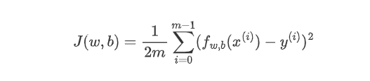 梯度下降算法:
 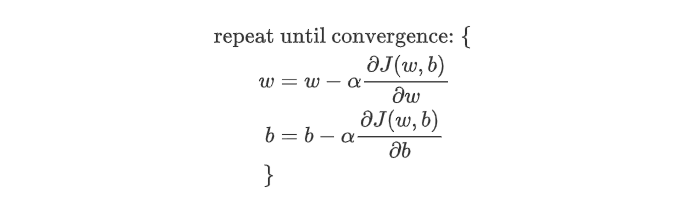 其中,α为学习率,决定单次下降的幅度。
梯度为: 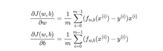
用代码实现:
1 | #计算误差函数 |
开始运行,示例:
1 | w_init = 1 |
Iteration 1000 Cost: 3.82e+00 dj_dw: -3.930e-01, dj_db:  6.358e-01 w:  1.946e+02, b: 1.08710e+02

Iteration 2000 Cost: 8.88e-01 dj_dw: -1.894e-01, dj_db:  3.065e-01 w:  1.974e+02, b: 1.04198e+02

Iteration 3000 Cost: 2.06e-01 dj_dw: -9.130e-02, dj_db:  1.477e-01 w:  1.987e+02, b: 1.02024e+02

Iteration 4000 Cost: 4.80e-02 dj_dw: -4.401e-02, dj_db:  7.121e-02 w:  1.994e+02, b: 1.00975e+02

Iteration 5000 Cost: 1.11e-02 dj_dw: -2.121e-02, dj_db:  3.433e-02 w:  1.997e+02, b: 1.00470e+02

Iteration 6000 Cost: 2.59e-03 dj_dw: -1.023e-02, dj_db:  1.655e-02 w:  1.999e+02, b: 1.00227e+02

Iteration 7000 Cost: 6.02e-04 dj_dw: -4.929e-03, dj_db:  7.976e-03 w:  1.999e+02, b: 1.00109e+02

Iteration 8000 Cost: 1.40e-04 dj_dw: -2.376e-03, dj_db:  3.844e-03 w:  2.000e+02, b: 1.00053e+02

Iteration 9000 Cost: 3.25e-05 dj_dw: -1.145e-03, dj_db:  1.853e-03 w:  2.000e+02, b: 1.00025e+02

(w,b) found by gradient descent: (199.9924,100.0122)
注意一下上面打印的梯度下降过程的一些特征。
成本开始很大,并迅速下降,如讲座中的幻灯片所述。
偏导数dj_dw和dj_db也会变小,一开始很快,然后越来越慢。如讲座中的图表所示,当过程接近 “碗底”时,由于该点上的导数值较小,所以进展较慢。
多元线性回归
使用到的python库:
1 | import copy,math |
问题陈述
你将使用住房价格预测的例子。训练数据集包含三个例子,有四个特征(尺寸、卧室、楼层和,年龄),如下表所示。 请注意,与先前的实验室不同,尺寸的单位是平方英尺而不是1000平方英尺。这导致了一个问题,你将在下一个实验中解决这个问题。
| 尺寸(平方英尺) | 卧室数量 | 楼层数量 | 房龄 | 价格(1000刀) |
|---|---|---|---|---|
| 2104 | 5 | 1 | 45 | 460 |
| 1416 | 3 | 2 | 40 | 232 |
| 852 | 2 | 1 | 35 | 178 |
记录数据
1 | x_train = np.array([[2104,5,1,45],[1416,3,2,40],[852,2,1,35]]) |
参数向量w,参数b
1 | b_init = 0 |
理论依据:
预测函数 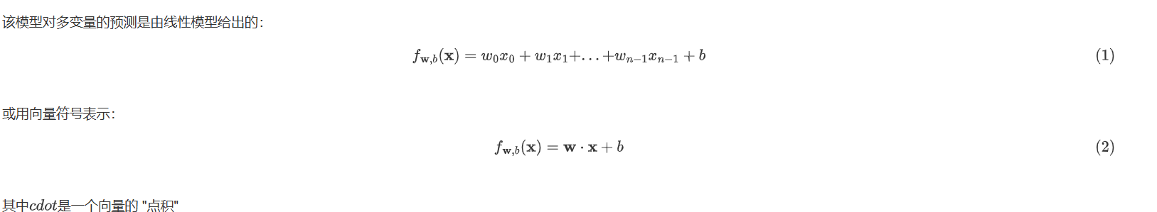
成本函数 
多变量梯度下降 
代码实现:
1 | import copy,math |
输出结果:
Iteration    0: Cost  2529.46
Iteration  100: Cost   695.99
Iteration  200: Cost   694.92
Iteration  300: Cost   693.86
Iteration  400: Cost   692.81
Iteration  500: Cost   691.77
Iteration  600: Cost   690.73
Iteration  700: Cost   689.71
Iteration  800: Cost   688.70
Iteration  900: Cost   687.69
最终找到的w为[ 0.2   0.   -0.01 -0.07],b为-0.00
预测值426.19,实际值:460

预测值286.17,实际值:232

预测值171.47,实际值:178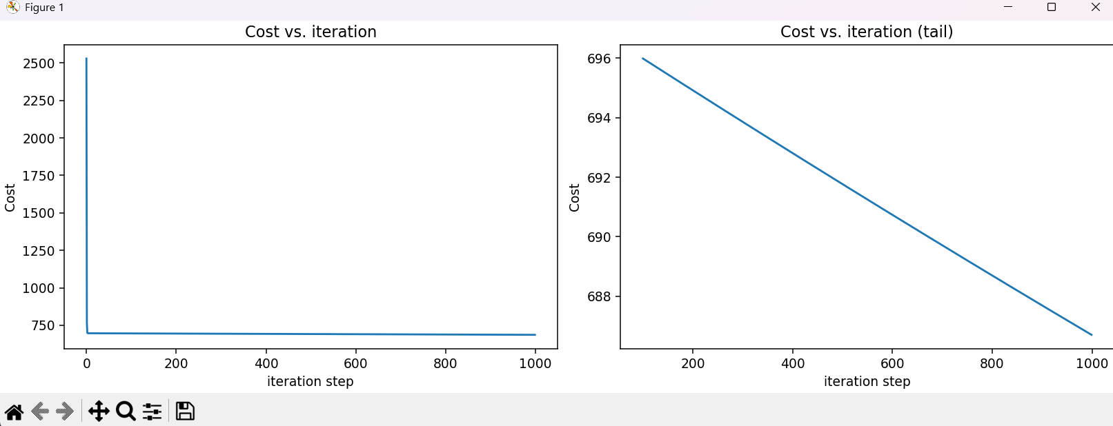
预测值和实际值地差别还是挺大的
解决办法:特征缩放 
代码实现:
1 | def zscore_normalize_features(x): |
现对x_train进行特征缩放,再进行梯度下降得到w,b
1 | x_norm,x_mu,x_sigma = zscore_normalize_features(x_train) |
Iteration Cost          w0       w1       w2       w3       b       djdw0    djdw1    djdw2    djdw3    djdb

---------------------|--------|--------|--------|--------|--------|--------|--------|--------|--------|--------|
        0 3.78405e+04  1.2e+01  1.2e+01 -4.1e+00  1.2e+01  2.9e+01 -1.2e+02 -1.2e+02  4.1e+01 -1.2e+02 -2.9e+02
      100 2.41945e-05  3.8e+01  4.2e+01 -3.1e+01  3.6e+01  2.9e+02  4.2e-05 -4.2e-05  6.3e-04  7.9e-05 -7.7e-03
      200 1.70488e-14  3.8e+01  4.2e+01 -3.1e+01  3.6e+01  2.9e+02  1.0e-09 -1.0e-09  1.5e-08  1.9e-09 -2.0e-07
      300 1.17254e-23  3.8e+01  4.2e+01 -3.1e+01  3.6e+01  2.9e+02  1.4e-14 -3.5e-14  3.7e-13  3.5e-14 -5.4e-12
      400 3.06962e-26  3.8e+01  4.2e+01 -3.1e+01  3.6e+01  2.9e+02  2.2e-14  2.0e-14  1.3e-14  2.3e-14 -2.5e-13
      500 3.06962e-26  3.8e+01  4.2e+01 -3.1e+01  3.6e+01  2.9e+02  2.2e-14  2.0e-14  1.3e-14  2.3e-14 -2.5e-13
      600 3.06962e-26  3.8e+01  4.2e+01 -3.1e+01  3.6e+01  2.9e+02  2.2e-14  2.0e-14  1.3e-14  2.3e-14 -2.5e-13
      700 3.06962e-26  3.8e+01  4.2e+01 -3.1e+01  3.6e+01  2.9e+02  2.2e-14  2.0e-14  1.3e-14  2.3e-14 -2.5e-13
      800 3.06962e-26  3.8e+01  4.2e+01 -3.1e+01  3.6e+01  2.9e+02  2.2e-14  2.0e-14  1.3e-14  2.3e-14 -2.5e-13
      900 3.06962e-26  3.8e+01  4.2e+01 -3.1e+01  3.6e+01  2.9e+02  2.2e-14  2.0e-14  1.3e-14  2.3e-14 -2.5e-13
w,b found by gradient descent: w: [ 38.05  41.54 -30.99  36.34], b: 290.00
现在来预测一个有1200平方英尺、3间卧室、1层楼、40年房龄的房子的价格。必须用训练数据归一化时得出的平均值和标准差对数据进行归一化。
1 | x_house = np.array([1200, 3, 1, 40]) |
输出结果:
predicted price of a house with 1200 sqft, 3 bedrooms, 1 floor, 40 years old = $281683


